Waterfall chart excel with multiple series
Now click on Insert Tab from the top of the Excel window and then select Insert Line or Area Chart. So basically the waterfall chart is using the pivot table as its source.
Excel Waterfall Charts My Online Training Hub
Double-click on one of the chart columns to bring up the Format Data Series pane.

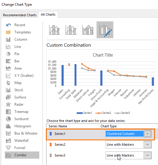
. Lets take an example of sales of a company. Another way to manage the data series displayed in your Excel chart is using the Chart Filters button. Change the default chart type for Series Planned Hours and Actual Hours and push them to the secondary axis.
It uses simple but unusual techniques to quickly and easily get a Waterfall Chart that also works with negative cumulative values. However we can add multiple series under the barcolumn chart to get the Comparison Chart. Following is an example of a doughnut chart in excel.
Beside each series is a dropdown showing its chart type and a checkbox showing its axis group. Displaying multiple time series in an Excel chart is not difficult if all the series use the same dates but it becomes a problem if the dates are different for example if the series show monthly and. Gantt Chart Examples.
I have a tutorial for regular waterfall charts. Brand new major upgrade. Click on the drop-down menu of the pie chart from the list of the charts.
To add a chart title in Excel 2010 and earlier versions execute the following steps. Right click on any series in the chart and choose Change Series Chart Type The dialog shows the chart with a list of series in the chart. Right click the chart and choose Select Data or click on Select Data in the ribbon to bring up the Select Data Source dialogYou cant edit the Chart Data Range to include multiple blocks of data.
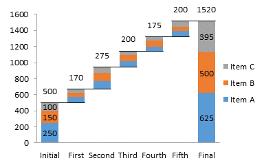
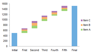
Create a Bubble Chart. If you use the stacked column approach a stacked waterfall has multiple items per category. Here we discuss its uses how to create a waterfall chart in Excel and Excel examples and downloadable Excel templates.
Click the Chart type dropdown in the Area series row and select Area or Stacked Area doesnt matter which in this case since theres only one area series. Click anywhere within your Excel graph to activate the Chart Tools tabs on the ribbon. From the pop-down menu select the first 2-D Line.
Click for 30 days free trial. If you can make it work with one set of values you should be able to add one or more extra series to stack on the first. This article is a guide to the Waterfall Chart in Excel.
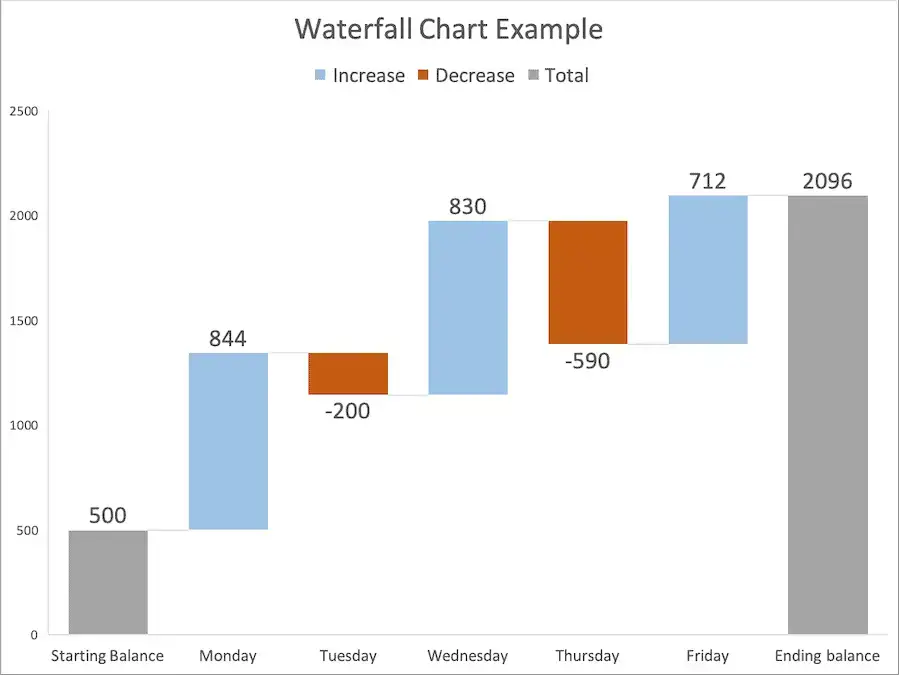
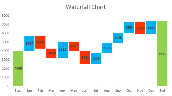
I also make one of those add-ins. Switch to the Combo tab. A waterfall chart also known as a cascade chart or a bridge chart is a special kind of chart that illustrates how positive or negative values in a data series contribute to the totalIn other words its an ideal way to visualize a starting value the positive and negative changes made to that value and the resulting end value.
You may also look at these useful functions in Excel. A Microsoft Excel template is especially convenient if you dont have a lot of experience making waterfall charts. There are more custom chart types and functions available and existing features have been enhanced.
Peltier Tech has been busy upgrading the powerful Charts for Excel add-in. It is a built-in chart type in Excel 2016. You can add one trendline for multiple series in a chart.
If your module does not say Option Explicit at the top type it in manually. With the help of a double doughnut chart we can show the two matrices in our chart. Then you can remove excess white spaces between the columns to make them stand closer to one another.
This button appears on the right of your chart as soon as you click on it. Bridge Chart Flying Bricks Chart Cascade Chart or Mario Chart. Watch the video to learn how to create a Waterfall or Bridge Chart in Excel.
Double Doughnut Chart in Excel. In the opened Format Data Series pane under the Fill Line icon select No fill and No line from the Fill and Border sections separately see. Creating Pie of Pie Chart in Excel.
On the chart itself right-click the line for either Series Planned Hours or Series Actual Hours. If you are a user of an earlier version of Peltier Tech Charts for Excel contact Peltier Tech for a coupon code. Transform the data series representing the planned and actual hours into a clustered column chart.
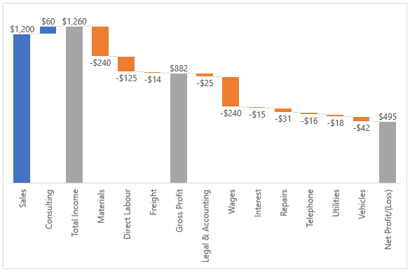
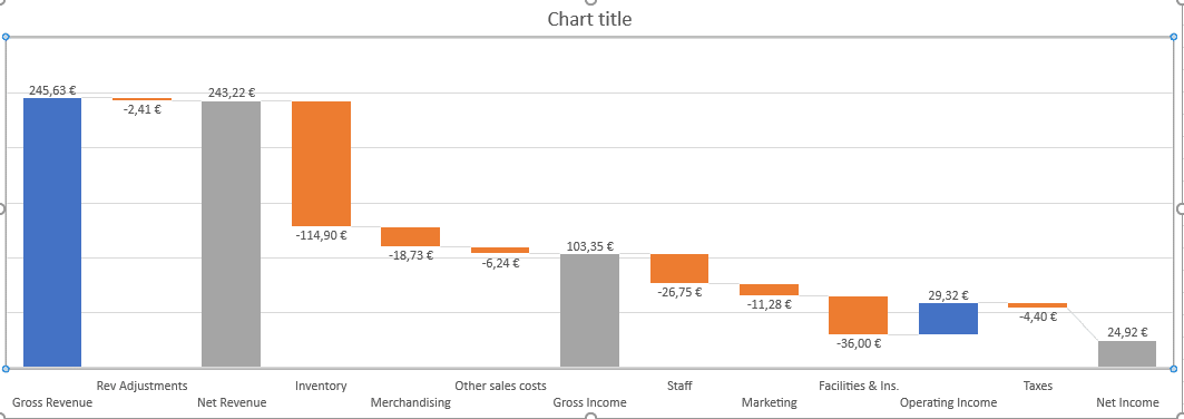
Excel Waterfall Charts Bridge Charts Conditional Formatting of Excel Charts. A Waterfall Chart visually breaks down the cumulative impact of sequential positive or negative values on a final outcome ex. Follow the below steps to create a Pie of Pie chart.
However you can add data by clicking the Add button above the list of series which includes just the first series. In some times to create or insert a complex chart such as milestone chart waterfall chart and so on need several steps. Waterfall charts 101.
I recently showed several ways to display Multiple Series in One Excel ChartThe current article describes a special case of this in which the X values are dates. If you prefer to read instead of. While in the Options dialog uncheck Auto Syntax Check.
Lets understand the Pie of Pie Chart in Excel in more detail. On the Layout tab click Chart Title Above Chart or Centered Overlay. Various income and expense items on the final profitability.
The Excel Chart SERIES Formula - Peltier Tech Blog says. Read about it below. The easiest way to assemble a waterfall chart in Excel is to use a premade template.
This will place Option Explicit at the top of every new module saving innumerable problems caused by typos. First add a hidden series that uses all of the X and Y values in the chart then add a trendline. To delete a certain data series from the chart permanently select that series and click the Remove bottom.
Hide or show series using the Charts Filter button. In Excel 2013 the Change Chart Type dialog appears. This then changes the data that feeds the waterfall chart.
From the pop-down menu select the first 2-D Line. In Excel Click on the Insert tab. A comparison chart is best suited for situations when you have differentmultiple values against the samedifferent categories and you want to have a comparative visualization for the same.
Tuesday September 24 2019 at 906 am. There is no chart with the name as Comparison Chart under Excel. Next you need to format the stacked column chart as a waterfall chart please click on the Base series to select them and then right click and choose Format Data Series option see screenshot.
Excel Waterfall Charts Bridge Charts. In the Change Chart Type tab go to the Line tab and select Line with. In the Change Chart Type dialog box transform the clustered bar graph into a combo chart.
Select Series Data. Then go to Tools Options and in the Editor tab check the Require Variable Declaration checkbox. Link the chart title to some cell on the worksheet.
Whenever a slicer item is selected the pivot table in cell M3 is filtered and the data in the pivot table changes. But if you have Kutools for Excels Auto text pane you just need to create the chart once time and add it as the auto text you can insert the charts to every sheet as you need in any time. All you need to do is to enter your data into the table and the Excel waterfall chart will automatically reflect the changes.
Right click on the Area series which is still of type XY and choose Change Series Chart Type. Doughnut Chart in Excel Example 2. I will update the file with a waterfall chart that is created manually so you can get this.
Change the Gap Width to something smaller like 15Close the pane. This is very easy with Excel 2013s new Change Chart Type dialog. Here we are considering two years sales as shown below for the products X Y and Z.
For Series Cumulative change Chart Type to Line with Markers and check the Secondary Axis box. Now select Pie of Pie from that list. Excel 2010 or older versions.
Add title to chart in Excel 2010 and Excel 2007.

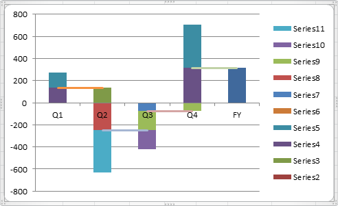
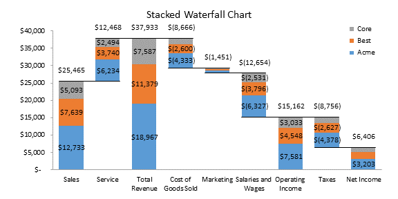
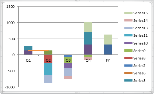
Stacked Waterfall Chart With Positive And Negative Values In Excel Super User
How To Create Waterfall Charts In Excel Page 5 Of 6 Excel Tactics
How To Set The Total Bar In An Excel Waterfall Chart Analyst Answers
Excel Waterfall Charts Bridge Charts Peltier Tech
How To Create Waterfall Chart In Excel 2016 2013 2010
Excel Waterfall Chart How To Create One That Doesn T Suck
Excel Waterfall Charts My Online Training Hub
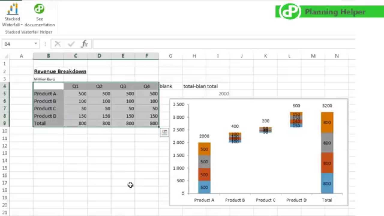
Stacked Waterfall Chart In 10 Seconds With A Free Add In For Excel Youtube
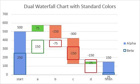
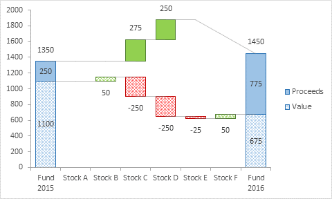
Peltier Tech Dual Waterfall Chart Peltier Tech Charts For Excel
Excel Waterfall Charts Bridge Charts Peltier Tech

Stacked Waterfall Chart Microsoft Power Bi Community
The New Waterfall Chart In Excel 2016 Peltier Tech
The New Waterfall Chart In Excel 2016 Peltier Tech
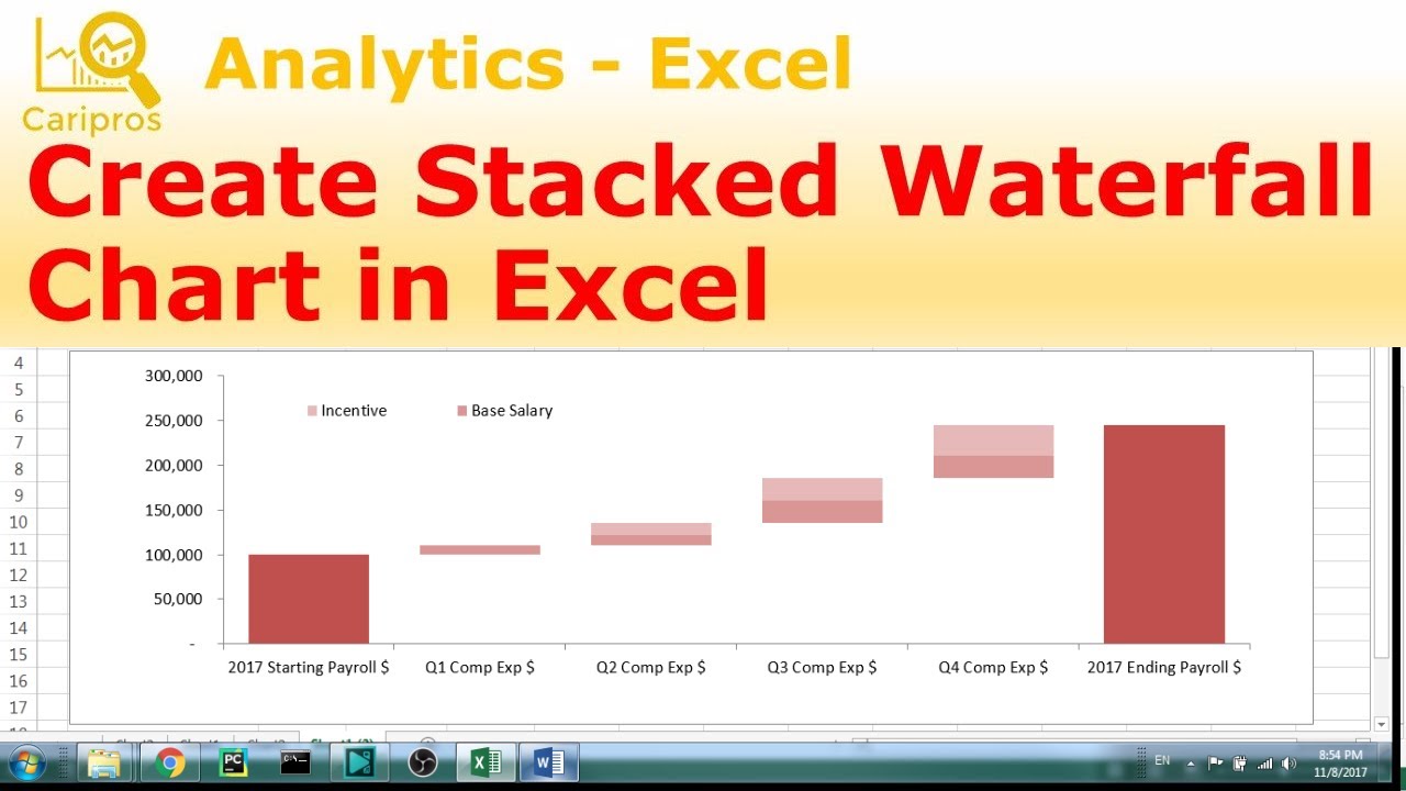
Excel Chart Stacked Waterfall Chart For Annual Expenses Reporting Youtube
How To Create Waterfall Charts In Excel Page 5 Of 6 Excel Tactics
Create Waterfall Or Bridge Chart In Excel
.png)
Waterfall Chart Excel Template How To Tips Teamgantt